Transformers : Understanding Queries, Keys, & Values and the Math behind it

Till now we understand how text is converted into final input matrix :

Text → Tokens → Token IDs → Embeddings → + Positional Encoding → Final Input Matrix

(if you didn’t read the previous part → Transformers : Builing Intuition)

We also know that transformers use self-attention mechanisms to process sequential data in parallel. But why do we need these self-attention mechanisms? It is because words often have more than one meaning and their meaning depends on the context of the sentence or the words surrounding that word in the sentence. So self-attention helps the model to get rid of ambiguities and understand how the word relates to the context.

So now let us understand how this works.

Every token has 3 roles: Query (Q), Key (K), and Value (V).

• Query → what is the word looking for
• Key → what does it contain
• Value → what info this word contributes

But we don't understand anything by the above definition. So now let's understand it mathematically.

Think of query, key, and value as separate vector spaces all together. These vector spaces are always projected into lower dimensions for faster computations that we will see below.

Take an example of the word "cat". Let's say the embedding of the word "cat" is: $x = [1,2,3,4]$. We want to project this into 2-dimensional Q, K, V vectors. For that we multiply the embedding of the token with some pre-learned weight matrices inside the transformer. Let's say the weights are $W_q$, $W_k$, and $W_v$. So,

Basically,

• $W_q$ : The matrix that transforms the token embedding into a Query vector
• $W_k$ : The matrix that transforms the token embedding into a Key vector
• $W_v$ : The matrix that transforms our token embedding into a Value vector

Each of these matrices is learned during training. So here in our example each of them will be a 4x2 matrix. For example let's pick simple numbers for illustration :

Wq = [ 1 0 , 0 1 , 1 1 , 0 1 ]
Wk = [ 1 1 , 1 0 , 0 1 , 1 0 ]
Wv = [ 0 1 , 1 1 , 1 0 , 0 1 ]

Now compute Q, K, V by multiplying x by each matrix :

• Q = $xW_q$ = $[ 1 , 2 , 3 , 4 ] [ 1 0 , 0 1 , 1 1 , 0 1 ] = [ 4 , 9 ]$
• K = $xW_k$ = $[ 1 , 2 , 3 , 4 ] [ 1 1 , 1 0 , 0 1 , 1 0 ] = [ 7 , 4 ]$
• V = $xW_v$ = $[ 5 , 7 ]$

(Here bias is also present but we have not included it for the sake of simplicity.)

So, embedding → raw meaning of token, and

$W_q$, $W_k$, $W_v$ → different lenses that highlight different aspects of that meaning.

Now that we have Q, K, and V vectors we will compute the attention score.

The attention score is the dot product of Query and Key transpose, i.e. basically finding the similarity between two vectors representing “What is the token looking for?” and “What does the token contain?” :

If we had multiple tokens, we’d compute this score between the Query of one token and the Key of every other token.

Now this score needs to be normalized by turning these into weights. For this we apply Softmax to this score. This Softmax converts the raw similarity scores into attention weights (probabilities) that sum to 1. Here in our example we have only one token so it will be converted to 1.

Finally, we use the attention weight to scale the Value vector. With weight = 1 (single token case):

With multiple tokens, each Value would be multiplied by its attention weight, and then summed to form the new representation.

Multi-Token Example: "The cat sat"

Now let us take another example to understand the multi-token case so we can understand how attention actually distributes across words.

Step 1: Embeddings
Suppose each token embedding is 4‑dimensional (to keep numbers small):

• “The” → $[1,0,1,0]$
• “cat” → $[0,1,0,1]$
• “sat” → $[1,1,0,0]$

Step 2: Project into Q, K, V
We’ll use simple weight matrices (size 4 x 2) and biases. After projection, we might get:

• “The”: $Q=[1,2]$, $K=[0,1]$, $V=[1,0]$
• “cat”: $Q=[2,1]$, $K=[1,0]$, $V=[0,1]$
• “sat”: $Q=[1,1]$, $K=[1,1]$, $V=[1,1]$

Step 3: Compute Attention Scores
For each word, we compare its Query with every other word’s Key (dot product):

• “The” attends to:
  • “The”: $Q\cdot K = [1,2]\cdot [0,1] = 2$
  • “cat”: $[1,2]\cdot [1,0] = 1$
  • “sat”: $[1,2]\cdot [1,1] = 3$
• “cat” attends to:
  • “The”: $[2,1]\cdot [0,1] = 1$
  • “cat”: $[2,1]\cdot [1,0] = 2$
  • “sat”: $[2,1]\cdot [1,1] = 3$
• “sat” attends to:
  • “The”: $[1,1]\cdot [0,1] = 1$
  • “cat”: $[1,1]\cdot [1,0] = 1$
  • “sat”: $[1,1]\cdot [1,1] = 2$

Step 4: Softmax Normalization
Convert scores into weights (probabilities). For example, for “The”:

• Raw scores: $[2, 1, 3]$
• Softmax → approx $[0.27, 0.10, 0.63]$

So “The” pays 63% attention to “sat,” 27% to itself, and 10% to “cat.”

Step 5: Weighted Values
Now each word’s new representation is a weighted sum of the Values. For “The”:

This means “The” is re‑represented in context, heavily influenced by “sat.”

To sum up:

• Q and K decide how much attention one word pays to another.
• Softmax ensures those scores become meaningful probabilities.
• V carries the actual information, which gets blended according to those weights.

So we started with “The”’s original value vector $[1,0]$ → blended it with contributions from “cat” $[0,1]$ and “sat” $[1,1]$, weighted by attention scores → The result is a new vector: $[0.90,0.73]$. This vector is the contextualized representation of “The”. It encodes information about how “The” relates to “cat” and “sat” in the sentence.

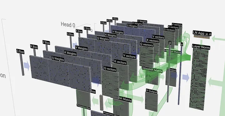
Multi-Head Attention

In practice, all of the things discussed above take place at once for the whole sentence instead of doing it token by token i.e. all tokens are processed simultaneously using matrix multiplication.

So far, you’ve seen:

Here, Q, K, V are produced by one set of weight matrices:

That’s one head: one way of projecting embeddings and computing attention.

In practice, transformers don’t stop at one head. They use multiple sets of weights:

Each head computes its own attention:

Then all heads are concatenated:

where $W^O$ is another learned matrix that mixes the heads together. With $W^O$, the model learns to integrate multiple perspectives into one unified representation.

We can think of each head as a different perspective or different aspect. By having multiple heads, the model can pay attention to different aspects of the sentence in parallel (syntax, semantics, positional relations etc).

import numpy as np

def self_attention(X, W_Q, W_K, W_V):
    
    # Step 1: Compute Q, K, V
    Q = X @ W_Q
    K = X @ W_K
    V = X @ W_V

    # Step 2: Compute attention scores
    d_k = Q.shape[-1]
    scores = Q @ K.T / np.sqrt(d_k)

    # Step 3: Softmax to get weights
    # (Assuming a simple softmax implementation exists)
    attention_weights = np.exp(scores) / np.sum(np.exp(scores), axis=-1, keepdims=True)

    # Step 4: Weighted sum of values
    output = attention_weights @ V

    return output, attention_weights